Climate Variability and Climate change

    The distinction between Climate variability and Climate change inevitably has a degree of arbitrariness and depends on the time frame considered

We can call the natural reversible semi periodic variations which are embedded in the mean state of Climate as Climate variability.

Climate variability is different from seasonal variability which complete its cycle within the period of one year.

some of the examples of climate variabilities are

Indian Ocean Dipole (2 to 3 year)
El-Nino Southern Oscillation (2 to 7 years)
Solar Cycle (about 11 years)
Atlantic Multidecadal Oscillation(AMO) (60 to70 year)
Precession(axis orientation) variation (23000 years)
Obliquity (axis tilt angle) variation (41000 years)
Eccentricity (Ellipticity of orbit ) variation (100000 years)

Mechanisms to which Climate is sensitive

1. Milankovich cycle (Astronomical cycle) are importent in the long term beyond centuaries

2. The solar constant variation is less than 0.1% definitely in the last 25 years, probably in the last century and possibly in the last million years.

3. Green house gases have experienced long term natural and recent anthropogenic changes. The warming effect of green house gases and cooling effect of sulphite aerosols explains the recent warming trend.

4. Deep Ocean Circulation changes can cause climate changes which require mere decades to significantly alter land and sea surface temperature. This has occurred in relatively recent past  of about 10000 years ago and may be possible if triggered by greenhouse warming.

5. The coupled ocean atmosphere system oscillates and produce inter annual and decadal variations in climate, which are predictable in some extend

6. Cloud radiation interaction is another important factor which have strong influence on climate. But no past data is available for the pre satellite era.

7. Land surface changes also have influence on climate but most of them are local and irreversible. One of the major example is the influence of Himalayas orography and Asian monsoon

 

Why the ocean current is elliptical with strong western boundary current?

1. The tropical easterly wind causes poleward Ekman transport and the midlatitude westerly wind causes equatorward Ekman transport.

2. The Ekman transport converges at the subtropics causes downwelling. The diverging region of Ekman transport cause upwelling.
(Reason: Continuity and conservation of mass)

3. The downwelling push the thermocline down and squeeze the underling geostrophic layer. The upwelling pull the thermocline up and stretches the geostrophic layer.
(Reason: Continuity and conservation of mass)

4. The squeezing causes equatorward Sverdrup transport and stretching lead to poleward Sverdrup transport.
(Reason: Potential vorticity conservation)

5. The equatorward Sverdrup transport diverges from the midlatitude westerly and converges to the tropical easterly forms an elliptical clockwise gyre in the interior layer of open ocean

6. This large scale equatorward mass transport is compensated by the poleward western boundary transport.
(Reason: Continuity and conservation of mass)

7. Thus the ocean current is elliptical with strong western boundary current.


Key words:

Atmospheric surface wind
Ekman layer mass transport
Potential vorticity
Geostrophic layer
Sverdrup transport

Text output of the data from GrADS

I want to take a text output of the data according to my need...I have already used one function "fprintf.gs" for this...It was a good tool.But It will not hep me as my data set is too big and it it is taking so much time to do it....So wats ur suggesion..How can i do it ?

You can use fwrite command with whichever variable you want to write.

fwrite Writes data to file instead of drawing a plot.

The syntax is as follows:

set fwrite fname
set gxout fwrite
display expression
disable fwrite

Here the output will be in Binary. But you need ASCII text output.



i want ascii

bcs this data i want to use for other softwares


Check the link
http://metoce.blogspot.com/search/label/get%20printout%20values%20as%20output?zx=98a27ead578a422a

yeah i used like that.. i modified by including latitudes and longitudes

but now tha problm comes

u given tt=tt+1...

here 1 is constant and giving the incriment

like that i want lat= lat+incriment

..but my lat have no constant incriment

How is the distribution of your lat-increment ? We shall try. Now the solution is very near.

but we cant say such a distribution

say...near to equator it is varying with 0.45 degress

while going to pole ..this incriment is decresing..but not in a specific order

But there should be some order either linear or nonlinear.

i have not find such an order. i want to have a close look for that. anyway linear order is not there. i can send the "ctl" file to u. so that u can have alook on the varying of my latitude.

It can be solved in GrADS. It is possible in two different ways.

1. If we can have ordinary one dimensional array variable in GrADS to store Latitude values and use it inside the loop.

2. If the philosophy of distribution of latitude is available from the documentation of the model, so that we can regenerate the latitude values using code.

Let us try the first way.

GrADS allows for arrays using the syntax varname.i.j (e.g., for a 2-D array), where i and j must be integers.

For our problem we need a one dimensional array to store latitude values.

let it be lt.i

First you assign all the latitude levels to the array lat.i
lt.1=your first level of latitude
lt.2=your second level and so on

Then use it in your loop by incrementing the counter variable i inside the loop.

Finally code become
--------------
--------------
--------------
while(tt<=tlimit)
'set t 'tt

while(i<=ilimit)
'set lat 'lt.i

while(ln<=lnlimit)
'set lon 'ln

'd variable'
te=subwrd(result,4)
w=write(fname.txt,te)

ln=ln+1
endwhile

i=i+1
endwhile

tt=tt+1
endwhile

'print'
---------------

As u suggested i wrote one script including the array dimension.
This is the final script I am sending...I could get the output now.

Any way pls see my final script( iam attaching herewith)

Thanks a lot

'reinit'
'open goa_may05_dom3_finalattempt.ctl'
'set lon 71.5087'
lat.1 = 13.23363
lat.2 = 13.25990
lat.3 = 13.28616
'set t 1'
count=1
while( count <= 2)
'set t ' count
longi = 71.5087
while(longi <= 75.4507)
'set lon ' longi
i=1
while(i <= 3)
'set lat ' lat.i
'd lat'
lrn=subwrd(result,4)
w=write('new_lat.txt',lrn)
i=i+1
endwhile
longi = longi+0.0270
endwhile
count=count+1
endwhile
'close 1'

Thanks for my friend seemanth to participate in this discussion

Climatology of season JJAS (grads script)

'reinit'
prompt 'Enter the name of new folder : '
pull fld
'!mkdir 'fld''
'open cmip1.ctl'
'q file'
'set lat -20 50'
'set lon 40 130'
'set time 1jun2022 30sep2101'
'define jjas=ave(prate, time=1jun, time=30sep)'
'set gxout shaded'
'd jjas'
'cbarn'
'define clim1=ave(jjas, time=1jun2022, time=30sep2101)'
'set time 1jun2022'
'd clim1*86400'
'set gxout shaded'
'd clim1*86400'
'cbarn'
'draw title cmip1 clomatology of JJAS'
'print climatology.gif'
'print 'fld'/clim1.eps'
'print 'fld'/clim1.gif'
'print 'fld'/clim1.jpg'
'!cd 'fld''
'!ls'

Some Beautifull Pictures

The Marks of Wind

Squall line

A squall line is a line of severe thunderstorms that can form along and/or ahead of a cold front. In the early 20th century, the term was used as a synonym for cold front. It contains heavy precipitation, hail, frequent lightning, strong straight line winds, and possibly tornadoes and waterspouts. Severe weather, in form of strong straight-line winds can be expected where the squall line in areas where the line itself is in the shape of a bow echo, in the portion of the line most bows out. Tornadoes can be found along waves within a line echo wave pattern, or LEWP, where mesoscale low pressure areas are present. Some bow echoes which develop within the summer season are known as derechos, and they move quite fast through large sections of territory. On the back edge of the rain shield associated with mature squall lines, a wake low can be present which are sometimes associated with a heat burst.



Lenticular Cloud


Lenticular clouds are stationary lens-shaped clouds that form at high altitudes, normally aligned perpendicular to the wind direction. Lenticular clouds can be separated into altocumulus standing lenticularis (ACSL), stratocumulus standing lenticular (SCSL), and cirrocumulus standing lenticular (CCSL).

Diffusion equation

The diffusion equation is a partial differential equation which describes density fluctuations in a material undergoing diffusion. It is also used to describe processes exhibiting diffusive-like behaviour, for instance the 'diffusion' of alleles in a population in population genetics.

The equation is usually written as:

where is the density of the diffusing material at location and time t and is the collective diffusion coefficient for density φ at location ; the nabla symbol represents the vector differential operator del acting on the space coordinates. If the diffusion coefficient depends on the density then the equation is nonlinear, otherwise it is linear. If is constant, then the equation reduces to the following linear equation:

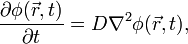
also called the heat equation. More generally, when D is a symmetric positive definite matrix, the equation describes anisotropic diffusion, which is written (for three dimensional diffusion) as:

Derivation

The diffusion equation can be derived in a straightforward way from the continuity equation, which states that a change in density in any part of the system is due to inflow and outflow of material into and out of that part of the system. Effectively, no material is created or destroyed:

,

where is the flux of the diffusing material. The diffusion equation can be obtained easily from this when combined with the phenomenological Fick's first law, which assumes that the flux of the diffusing material in any part of the system is proportional to the local density gradient:

.

Historical origin

The particle diffusion equation was originally derived by Adolf Fick in 1855.

Discrete analogs

The diffusion equation is continuous in both time and space. One may discretize space, time, or both space and time, which arise in application. Discretizing time alone just corresponds to taking time slices of the continuous system, and no new phenomena arise. In discretizing space alone, the Green's function becomes the discrete Gaussian kernel, rather than the continuous Gaussian kernel. In discretizing both time and space, one obtains the random walk.

List of candidates selected for the award of SPM Fellowship-2009

(Interviews held on 13th & 14th July 2009)



SNo
Roll No.
Name of the Candidate
Subject

1
114473
CHANDRABALI BHATTACHARYA
Chemical Sciences

2
115334
SATYAJIT GUPTA
Chemical Sciences

3
199351
KRISHNANKA SHEKHAR
Chemical Sciences

4
116453
PROSENJIT DAW
Chemical Sciences

5
116728
SOURAV KUMAR DEY
Chemical Sciences

6
CY7110754
DIPAK SAMANTA
Chemical Sciences

7
501422
SUPRIT SINGH
Physical Sciences

8
506733
RUDRANEL BASU
Physical Sciences

9
508448
KOLEKAR SANVED VINOD
Physical Sciences

10
505280
GOKHALE SHREYAS SHASHANK
Physical Sciences

11
327558
NEELANJANA J
Life Sciences

12
318092
SUMIT SEN SANTARA
Life Sciences

13
327145
WAREED AHMED
Life Sciences

14
330265
VIDHI MATHUR
Life Sciences

15
301959
SAKSHI ARORA
Life Sciences

16
XL8280315
PRIYANKA BAJAJ
Life Sciences

17
328230
NEHA NANDWANI
Life Sciences

18
409780
SUBHAMAY SAHA
Math. Sciences

19
404927
B RAVINDER
Math. Sciences

20
201132
KASTURI BHATTACHARYYA
Earth Sciences

21
201500
TAMOGHNA ACHARYYA
Earth Sciences

Source: http://csirhrdg.res.in/SPMF09result.htm
----------------------------------------------------------------------------
Shortlist before core committee interview
http://csirhrdg.res.in/spmf09%20final%20shortlisted.pdf